The OSNACA Project (Ore Samples Noramlised to Average Crustal Abundance) is an “open source” project where assay data are freely available online. Representative ore samples from all over the globe are being donated to the project and assayed at Bureau Veritas’ Ultratrace Laboratory in Perth. All funds contributed by industry go towards analytical costs. The assay suite includes 65 ore, pathfinder, major and lithogeochemical elements.
Almost all elements are analysed to a detection limit at, or below, average crustal abundance. The assay database is backed by a library of reference samples and laboratory pulps stored at the CET. These materials are publicly available for further study including additional geochemical analyses and microscopy. Initial research on the data by CET staff and their collaborators is focused on multi-element ore signatures. A new technique has been developed that quantifies differences in multi-element signatures and makes it possible, for the first time, to create a map of “magmato-hydrothermal space”. The co-ordinate system of magmato-hydrothermal space is defined by the number of metallic elements included in a particular investigation. For example, 24 elements define a 24-dimensional mathematical space where each ore sample’s signature is defined by its “enrichment vector”.
The geochemical database being created by the OSNACA Project is critical in this regard because this mathematical approach requires an assay value for every element for every sample. No other publicly available dataset fulfils this requirement. It is recognised that the data has many other potential uses, hence the inclusion of major elements and a wide range of lithogeochemical elements. It is up to geoscientists from around the world how these data are to be used.
Ore samples are crushed in a steel jaw crusher with barren quartz processed between each sample. They are then pulverised to -75µm in a steel mill, with barren quartz rinse milled in between each sample.
Analytical solutions for reading by ICP-MS and ICP-OES are prepared by the following methods
1 Pb Fire assay Au, Pt, Pd
40 grams of sample is weighed (lower weights down to 10 grams can be used if there is insufficient sample or for highly sulphidic samples). The sample is then fused for one hour at 1100 oC in a ceramic pot with 165 grams of flux (a mix of borax , soda ash, flour ,litharge and a small amount of Silver ) with additional soda ash for silica rich samples, additional borax for basic samples, and additional KNO3 and litharge for some sulphidic samples. During the fusion the litharge( PbO) is reduced to Pb collecting the precious metals. Molten samples are poured into steel conical moulds where a lead button sinks to the bottom separating from the glass slag. The lead button is then placed on a cupel and heated to 990 oC for 45 minutes during which time the Pb oxidises back to PbO flowing into the absorbent cupel leaving behind a silver prill containing all Au,Pt & Pd. The prill is then dissolved in 1 ml of concentrated nitric acid followed by 1 ml of concentrated hydrochloric acid at 110 oC. The resultant solution is then made up to 10 ml with deionised water.
2 Peroxide Fusion B, Cr, Hf, Pb, S, Sb, Si, Sn, Ta, Ti, W, Zr
0.2500 grams of sample is fused with 1.5 g of Sodium Peroxide in an alumina crucible for 30 minutes at 650 oC. For Carbon rich samples the temperature is raised slowly to 650 oC to allow ashing for 1 hour prior to fusion. The crucible is allowed to cool and then agitated in 100 ml of deionised water for one hour, before adding 100 ml of hydrochloric acid and agitating every 10 minutes for 30 minutes in a waterbath at 95 oC. The solution is made up to 500 ml with de-ionised water.
3 Aqua Regia Au, Bi, Te, Hg, Ag, Sb
4.000 grams of sample is placed in a polythene vial before 5 ml of concentrated nitric acid is added in 1 ml increments checking for violent reactions before agitating and adding a further 5 ml of nitric acid. 10 ml of concentrated hydrochloric acid is added, agitated, and left to stand for 30 minutes before heating to 95 oC for two hours in a waterbath. The solution is made up to 50 ml with deionised water.
4 Mixed Acid (Hot Box) Ag, Al, As, Bi, Ca, Cd, Co, Cs, Cu, Fe, In, K, Li, Mg, Mn, Mo, Na, Nb, Ni, P, Pb, Rb, Re, Sc, Se, Sn, Sr, Te, Th, Tl, U, V, W, Y, Zn, REEs
0.1500 grams of sample is placed in a teflon tube and dissolved in 10 ml of a concentrated mixture of hydrofluoric, nitric and perchloric acids (hot-box mix). This solution is brought up to 250 oC and back down to 150 oC over a period of 12 hours. After allowing to cool for 5 minutes, 10 ml of concentrated hydrochloric acid is added and the sample is re-heated to 150 oC for 15 minutes. 10 ml of de-ionised water is added before decanting into a polystyrene tube. The solution is made up to 20 ml with deionised water and mixed thoroughly by agitating.
Whole rock geochemical data are presented as raw laboratory files, and in tabular format that can be linked with metadata by sample number. In the tabular data files, a “preferred value” has been selected for those elements which have been analysed by two different techniques; a robust and a sensitive technique. For the element tabulated below, the robust technique ensures complete digestion for samples that contain high concentrations, and the sensitive technique allows readings to lower detection limits where concentrations are low. The “robust cut-off” is the value below which the sensitive technique is used in preference to the robust technique. Combining the data in this way ensures the most reliable value for each of these elements over a very wide range of concentrations.
| Element | Robust Technique | Robust LLD (ppm) | Robust cut-off (ppm) | Sensitive Technique | Sensitive LLD (ppm) |
| Ag | Mixed Acid | 0.5 | Lab selected | Aqua Regia | 0.05 |
| Bi | Mixed Acid | 0.1 | Lab selected | Aqua Regia | 0.02 |
| Te | Mixed Acid | 0.2 | Lab selected | Aqua Regia | 0.02 |
| Pb | Peroxide Fusion | 100 | <1000 | Mixed Acid | 1 |
| Sb | Peroxide Fusion | 2 | Lab selected | Aqua Regia | 0.02 |
| Sn | Peroxide Fusion | 5 | <5 | Mixed Acid | 1 |
| W | Peroxide Fusion | 5 | <5 | Mixed Acid | 0.5 |
For Bi, Te, Ag and Sb a lot or repeat assaying was performed, particularly for samples that followed samples with very high values. Fusion, mixed acid and aqua regia data were all considered before selecting the preferred value. In general, mixed acid data for Ag and fusion data for Sb were found to be reliable right down to their respective detection limits, whereas aqua-regia data have been preferred for Bi and Te at values up to five times the mixed acid detection limit. Very high results for Ag, Bi and Te have been confirmed by fusion.
Bureau Veritas – Ultratrace have confirmed data for many other elements by comparing values by different techniques. These internal checks show, for example, that the REEs have been fully digested by the mixed acid technique when the data are compared to peroxide fusion data. Gold has been analysed by fire assay and aqua-regia to the same detection limit and fire assay values are used in preference.
For those interested in more information on data selection for Ag, Bi, Te and Sb (particularly those values that have not been published) further details can be provided by Alex Christ from Bureau-Veritas alex.christ@au.bureauveritas.com.
Selected geochemical data can be downloaded using the link below. The process of selecting a single “preferred value” for every element is explained in the “Data Selection” section of OSNACA Analytical Methods.
Link to OSNACA Data
Descriptions of the ore samples can be downloaded using the link below. Sample description can be linked to geochemical data using the sample number field common to each file (first column in each file).
Link to OSNACA Metadata
For those workers who would prefer to work with the original data from Bureau Veritas – Ultratrace, the original laboratory files can be downloaded below.
Link to Bureau Veritas Files

In kind sponsor
DONATIONS
Private individuals and corporations are invited to donate ore samples and/or funding to the OSNACA Project. The open source nature of the OSNACA Project and its tax-deductible status for financial donors is explained in the original OSNACA Formal Proposal.
Link to OSNACA Formal Proposal
We are extremely grateful to our foundation sponsors for their generous financial contributions. They responded positively to the initial circulation of the OSNACA Formal Proposal document in 2011. If you, or your company, would like to join them and donate funds to the OSNACA Project follow the link below.
Link to OSNACA Donation Form
If you have samples of unweathered ore-grade material from any significant ore deposit, we would be delighted if you made this material available to the OSNACA Project. Full details on how to select appropriate samples and what metadata also need to be provided are given in the link below. Please read the instructions on the “Instructions” worksheet carefully. It is the first page you will see when you open the file.
Link to OSNACA Sample Capture


The OSNACA mathematical technique quantifies differences in multi-element signatures and makes it possible to create a map of “magmato-hydrothermal space”. The co-ordinate system of magmato-hydrothermal space is defined by the number of metallic elements included in a particular investigation. For example, 24 ore and path-finder elements define a 24-dimensional mathematical space where each ore sample’s signature is defined by its “enrichment vector”. Every sample must be analysed for every element used in the calculations.
Raw data are normalised to average crustal abundance (ACA) after replacing all values below ACA with ACA. The normalised data are then logged and scaled to a fixed distance from the origin. This process is illustrated in two dimensions below
Data below ACA are replaced with ACA so that it is only metal enrichments that are measured. In other words, the analysis is restricted to the positive quadrant of Figure AA with average crustal abundance at the origin. Metal abundances below average crustal abundance may represent metal leaching but they may also represent the absence of this metal in the host rock to start with. In neither case is it desirable for this low metal abundance to affect the direction of the enrichment vector.
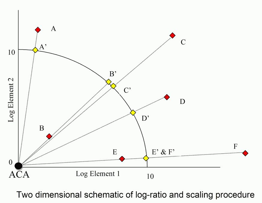
Log normalised data are scaled to a fixed distance from the origin (10 units) by dividing the vector by its length and multiplying by 10. With all data a fixed distance from the origin in 24-dimensional space, the Euclidian distance between any two sample points is a proxy for the angle between their enrichment vectors. Samples with similar metal signatures lie in similar directions from the origin, and have commensurately small Euclidian distances between scaled sample points. Dissimilar samples have large angles and commensurately large Euclidian distances between scaled data points.
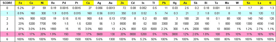
For elements with relatively high average crustal abundance (e.g., Cu (29 ppm) and especially Fe (56,000 ppm)) log10 measurements unduly restrict the log normalised score that these elements can reach (Fig. 2). Even for an abundance of 100% Fe, the log10 score is only 1.3. Therefore, for elements with ACA greater than 1 ppm, the base used to calculate the log normalised score has been adjusted so that 100% metal abundance gives a score of 6 (Fig. 3, Table 1). For elements with ACA below 1 ppm, scores higher than 6 have been “cut” to a value of six.

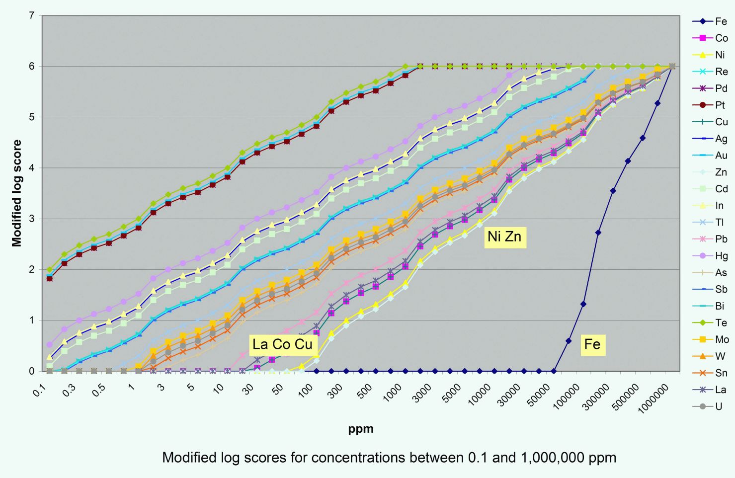
The resultant axes spread ore and path-finder geochemical values over a log score range of zero to six, in such a way that enrichment in one element can reasonably be compared to that of any other element. In Table 1, scores of 1 are universally recognised as “anomalous” in most ore environments, scores of 3 are around “ore grade”, and scores of 5 are universally regarded as “bonanza” grades. It is recognised that “ore grade” is an economic parameter that varies according to many factors but the attraction of this framework is its universality. It provides a fixed reference frame with which to quantify the difference between any two ore samples.
A worked example of the mathematical technique described above is provided in two downloadable files. Orogenic INPUT contains data for 79 Orogenic and Intrusion Related gold samples from the OSNACA database. The worksheet “Data” contains the raw data and all of the calculations through to scaled-log-normalised values. The worksheet “Matrix” calculates the Euclidean distance between every sample pair based on their scaled-log-normalised values. This matrix is the input for Hierarchical Clustering.
Hierarchical Clustering has been performed using the MultiDendrograms software package which can be downloaded free from the internet. The Joint Within Between algorithm was chosen to classify the samples.
Orogenic OUTPUT contains the same data for the 79 Orogenic and Intrusion-Related Gold samples but the samples have been ordered according to the results of Hierarchical Clustering. The dendrogram output is shown on worksheet “Dendrogram” where seven main groups (A-G) have been identified. The matrix on the worksheet “Matrix” shows the same groups and they are also plotted as spidergrams (worksheet Spidergrams) where the element enrichments that have led to these samples being grouped can be assessed visually.
The first division on the dendrogram is between Groups A-C (low As-Sb) and Groups D-G (high As-Sb). All of the intrusion related gold samples are in Groups A-C. Group A is distinct on the basis of elevated Cu and Bi ± Mo. Group B contains elevated Ag and Hg ± Mo, and Groups C contains elevated Bi ± Mo
Group D comprises samples that are not particularly closely related. This can be seen on the matrix and the spidergram. In contrast, Groups E and G form coherent spidergram patterns with commensurately small Euclidean distances between samples within each group. Groups E-G are marked by a fairly similar Au-As-Sb-Te-W signature.
A matrix for 872 ore grade samples, that has been organised according to hierarchical clustering is available as a downloadable file; OSNACA 2018 Poster, but requires an A0 plotter to print. It clearly demarcates distinct ore types such as Ni-Cu-PGE, Porphyry Mo and Sn mineralisation. It also separates different types of base metal deposit, different types of intrusion related deposits and a number of orogenic gold classes. Within each of the broad classes there are nested groups of more closely related samples (e.g., Zn-rich & Cu-rich VHMS deposits. Naturally, there is overlap between different ore classes and there are also some samples which have been widely separated by hierarchical clustering that have relatively small Euclidean distances between them. These samples can be identified on the matric by coloured cells a long way from the matrix diagonal. Clusters of like metal signature are plotted together on OSNACA enrichment plots where the nature of the metal signature can be visualised.